Vehicular optimal control problems have drawn attention for nearly a century, and are formulated today for hybrid vehicles and energy recovery systems. Solving them accurately for Formula One cars runs into a specific obstacle: there was no general method to obtain the geometric parameters of an F1 track in a form the solver could use.
That was the gap my undergraduate thesis filled.
Why the curvature is the blocker
The research this work supported — Limebeer, Perantoni and Rao’s work on optimal control of F1 energy recovery systems — applies direct orthogonal collocation to racing problems, with a more realistic aerodynamic model than earlier attempts and a focus on Kinetic Energy Recovery Systems.
That vehicle and aerodynamic model uses the curvature of the track as a function of distance travelled along it to compute where the car is. Which meant that without a way to calculate track curvature, minimum lap times simply couldn’t be computed for different circuits. Minimum-lap-time problems have been attacked as two-point boundary value problems, by direct transcription, and with linear optimal control techniques — but all of them need the track geometry first.
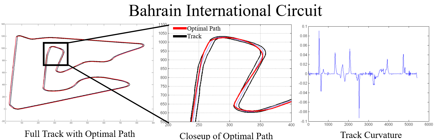
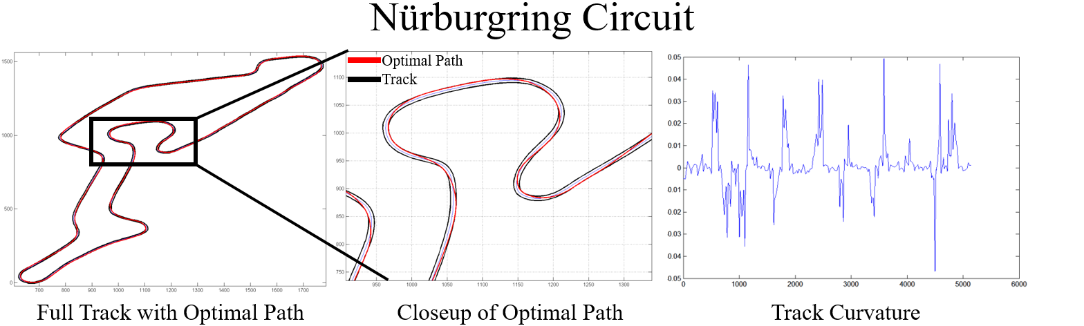
So the goal: take a user-picked image of any F1 track, calculate the centerline position and the curvature as a function of distance from the start line, and hand those to the existing GPOPS-II model. Deliberately user-friendly, and easy to follow.
From a picture to a centerline

The program accepts a black-and-white PNG or JPEG of the track. Source maps can come from Wikipedia or OpenStreetMap, converted with GIMP.
From there, MATLAB’s Image Processing Toolbox does the work:
imfillcloses the holes — sets of background pixels that can’t be reached by filling inward from the image edgebwareaopenremoves connected components under 50 pixels, then the small remaining holes are identified and filled by adding those pixel locations back to the imageskelandshrinkmorphological operations thin the filled track to a single line without letting it become discontinuous, and eliminate the stray “branches” left on the boundary
Then the racing direction: the user picks the start/finish line and the direction of travel,
and bwboundaries traces the centerline from that point, returning x-y coordinates in
the order a car would drive them. Local regression smooths out residual kinks.
Why splines were necessary
JPEG and PNG files are imperfect, so the binary centerline shows irregularities exactly where the track is supposed to be dead straight. The fix is to convert the centerline into smooth parametric equations.
The user either picks points along the track by mouse — which are then snapped to the nearest actual centerline points, since nobody clicks precisely — or lets the program take every nth point automatically, defaulting to every seventh.
Two coordinate corrections are needed at this stage. MATLAB indexes images with an inverted y-axis, so y values are subtracted from the maximum to make the plotted track appear upright rather than upside down; and the x values are negated to match the plotting convention in Limebeer’s work.
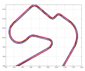
Distance along the track comes from a cumulative sum of the linear distances between a finely spaced set of points, with a nearest-neighbour search matching each user-selected point to its distance from the start line. With distance as the independent variable, spline equations for x and y follow — and those give a perfectly smooth centerline, free of the artefacts the source image introduced. A known distance scale on the track image converts pixels to metres.
Curvature, via Menger
Curvature is computed with Menger’s formula — the curvature is the reciprocal of the radius of the circle passing through three distinct points in n-dimensional Euclidean space. Distance along the track and curvature at 1000 points are saved under the variable names GPOPS-II expects.
Does it work?
Five circuits, run through the pipeline and then through the minimum-lap-time solver:
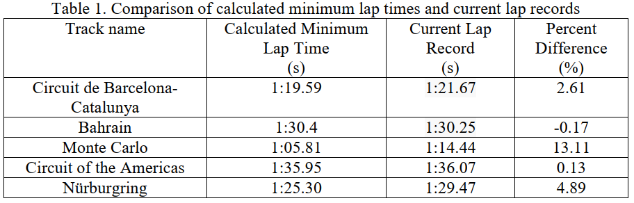
| Circuit | Calculated | Lap record | Difference |
|---|---|---|---|
| Circuit of the Americas | 1:35.95 | 1:36.07 | 0.13% |
| Bahrain | 1:30.40 | 1:30.25 | −0.17% |
| Barcelona-Catalunya | 1:19.59 | 1:21.67 | 2.61% |
| Nürburgring | 1:25.30 | 1:29.47 | 4.89% |
| Monte Carlo | 1:05.81 | 1:14.44 | 13.11% |
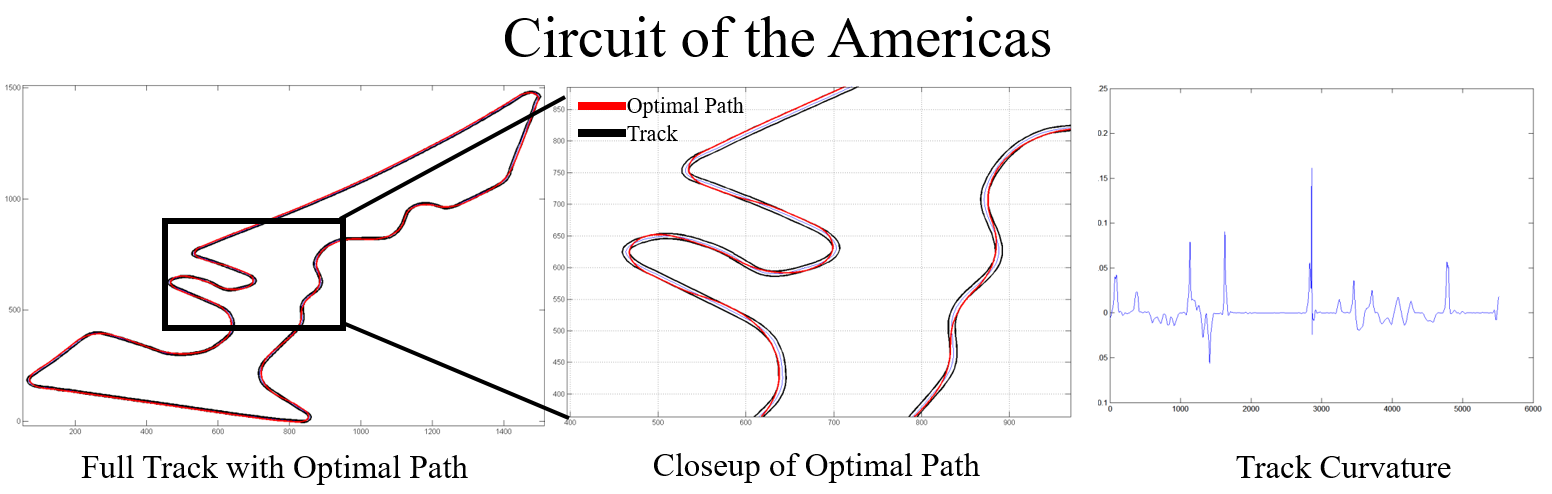
Two circuits land within a fifth of a percent of the real lap record, which is a strong result for a lap time computed from nothing but a picture of the track.
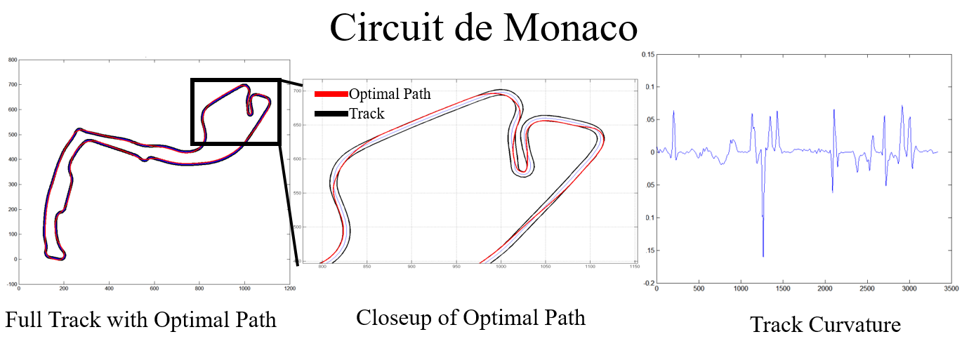
The spread at the other end is informative too. Monaco is the outlier by a wide margin — and it is the circuit where the assumptions bite hardest: a tight, low-speed street course where the ideal conditions the model assumes are least like reality, and where the fine detail of the image processing matters most to the extracted curvature.
References
- Limebeer, D. J. N., Perantoni, G., and Rao, A. V., “Optimal Control of Formula One Car Energy Recovery Systems,” International Journal of Control, Vol. 87, No. 10, Oct. 2014, pp. 2065–2080
- Patterson, M. A., and Rao, A. V., GPOPS-II Version 2.0, 2014 — uses the Radau Pseudospectral Method with collocation at the Legendre-Gauss-Radau points
- Léger, J., “Menger Curvature and Rectifiability,” The Annals of Mathematics, Vol. 149, No. 3, 1999, p. 831
- Track maps from Wikipedia and OpenStreetMap, processed with GIMP