GRAC — Compliant Robotic Leg — Rachel Hoffman-Bice, PhD

A single robotic leg with a motor at the knee and another at the ankle, riding a vertical guide rail so every drop is repeatable. The question was how to make it land softly: how much the joint stiffness and damping matter, and how much the leg’s angle at touchdown does.

The question

Landing after a jump is harder than it looks. If the leg joints are too stiff the landing is jarring, like running on concrete without padded shoes. If they are too compliant the leg wastes energy absorbing more impact than it needs to. People can’t easily keep some joints relaxed while tensing others on the way down, but a robot can hold any combination of independent joint stiffness and damping. So a robot can go looking for ratios for a quiet, controlled landing that biological legs can’t reach. We set out to test that, with a focus on how much the ankle contributes.

The leg

The leg has a femur, tibia and foot, with a DC motor and encoder at the knee and at the ankle, all hanging from a carriage on a guide rail with its own encoder. It drops onto a rubber pad. An MBED FRDM-K64F microcontroller runs the joint control loops, reading current sensors and an IMU, with MATLAB on the other end for commanding runs and logging data.

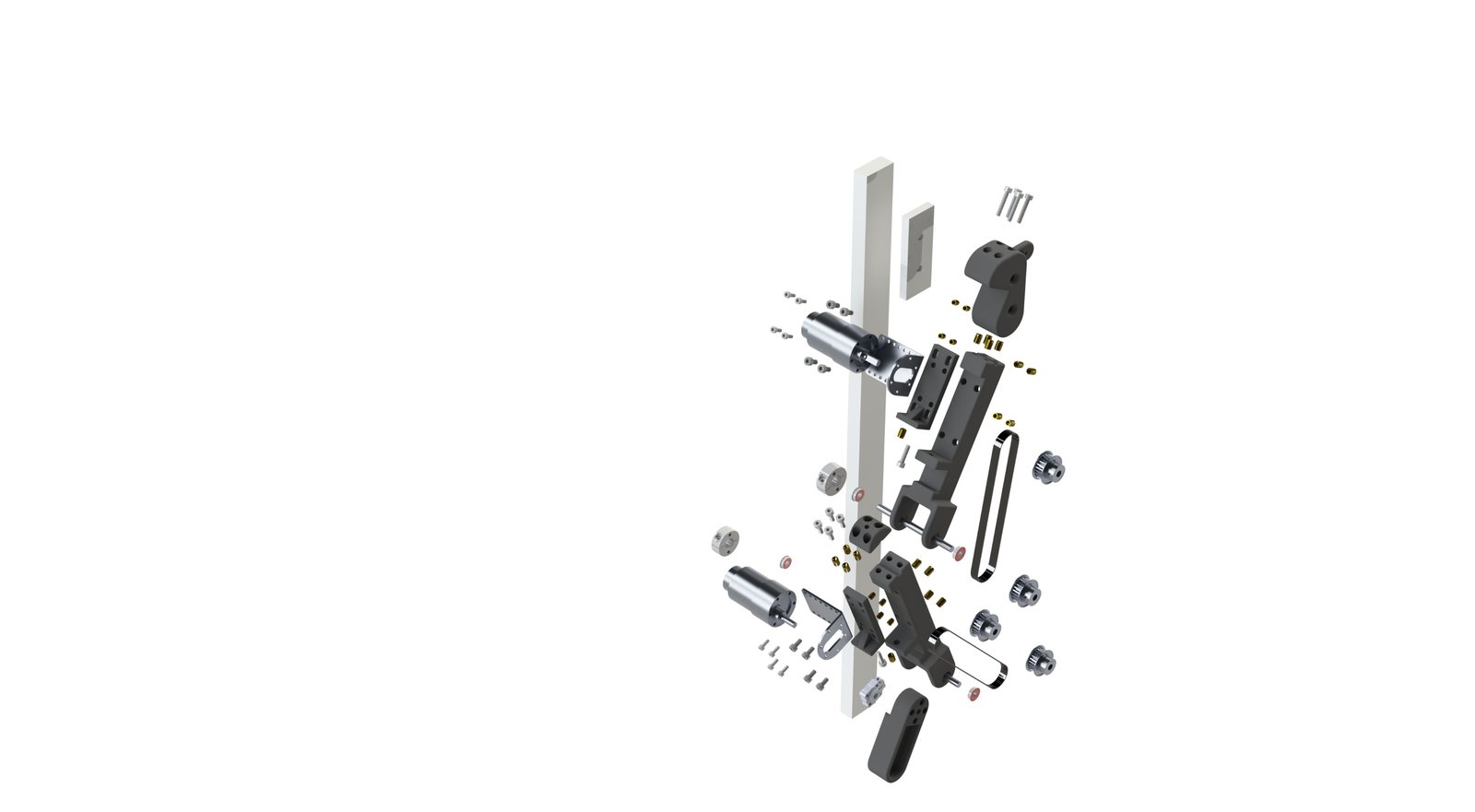
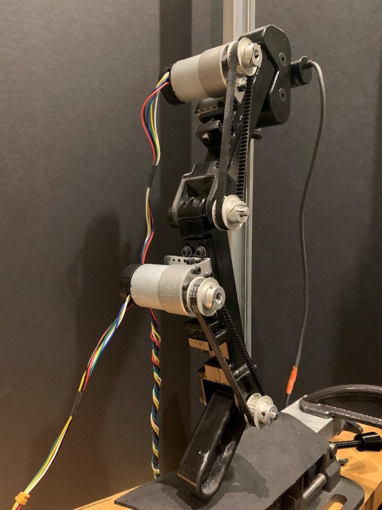
Exploded CAD of the leg on its guide rail: the rail carriage and adapter at the top, then femur, tibia and foot, with the knee and ankle motors, timing pulleys, bearings and fasteners pulled out along their axes

The built leg standing upright: black 3D-printed femur and tibia links, two gearmotors, and a timing belt running down to the ankle

The design changed along the way, and the three CAD revisions in the repo record it. An earlier version put a music-wire torsion spring at the ankle, a true series elastic joint. The final build drives both joints with motors instead and makes the compliance in software: each joint runs an impedance controller,

current_des = (-K * (angle - angle_des) - D * velocity + nu * velocity) / k_emf

so the stiffness K and damping D became numbers we could change between drops, with nu compensating for friction, instead of parts we had to swap.

The simulation (my part)

I built the model we used to decide what to test. The leg is a Lagrangian system with state q = [y, θ_knee, θ_ankle] and joint torques u = [τ_knee, τ_ankle] as inputs. The carriage only moves vertically and the hip angle is fixed, matching the rail. Each joint runs the same impedance law as the hardware. Ground contact is a spring-damper model with friction, and landing is simulated as a hybrid system: flight, the impact event and stance are separate regimes with a guarded switch between them rather than one integration straight through.

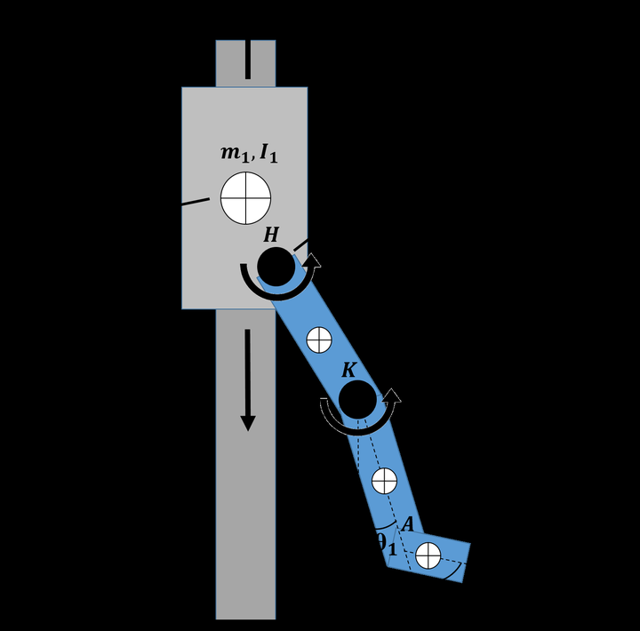
Model of the leg on the rail: the carriage of mass m1 on the vertical rail, with the hip H, knee K and ankle A joints marked on the leg below it

The dynamics are derived symbolically: Derive_everything_GRAC.m generates the mass matrix, Coriolis and gravity terms, energy, foot Jacobian and keypoint positions as MATLAB functions in AutoDerived/, and everything downstream (simulation, sweeps, animation) calls those. Jerk at the centre of mass comes from differentiating its trajectory twice.

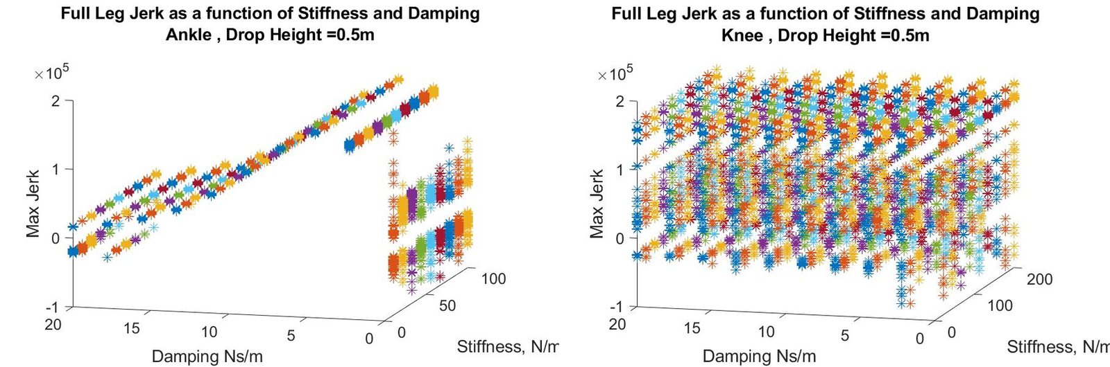
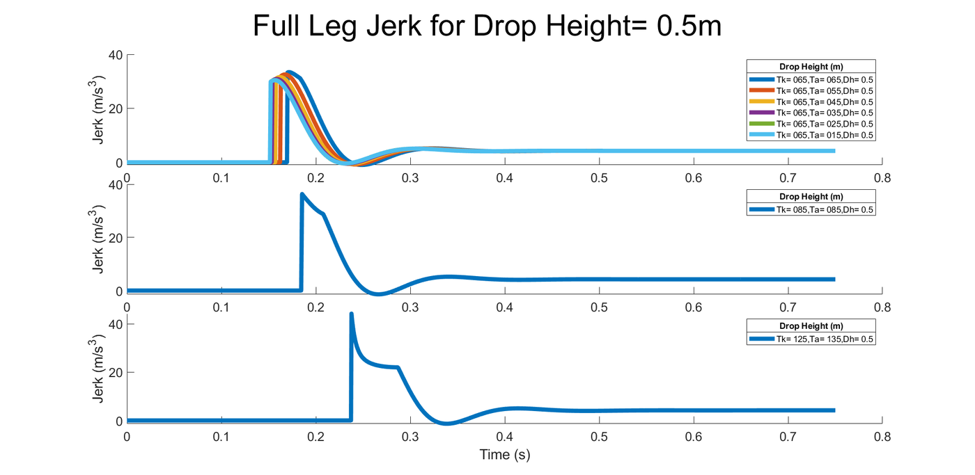
With that in place I swept everything we could control: knee and ankle stiffness and damping, the angle of attack at touchdown, and drop heights from 0.5 to 1 m. A configuration only counted if the leg didn’t collapse.

Simulation, 0.5 m drop, slowed 3×. Left: the joint gains that gave the lowest peak jerk. Right: the gains that gave the highest. The two landings are hard to tell apart.

Simulation, 0.5 m drop, slowed 3×. Left: a folded leg (knee 125°, ankle 135°). Right: a more extended leg (knee 65°, ankle 15°). The angle of attack changes the landing far more than the gains do.

Two 3D scatter plots of peak jerk against damping and stiffness for a 0.5 m drop, one sweeping the ankle and one the knee: the points form planes with no clear valley, showing gains have little effect on peak jerk

Jerk against time for full-leg simulations from a 0.5 m drop: each run shows a single sharp spike at touchdown that settles within about 0.1 s

Dropping the real leg

On the hardware we ran the same kind of sweep: set the gains and angle of attack, lift the carriage, let go, and log the encoders and IMU through the landing.

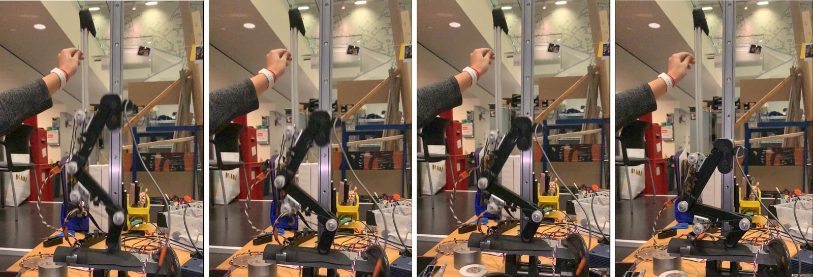
Four frames of a drop test: a hand lifts the leg up the guide rail and releases it, and the leg falls and lands on the pad with the knee flexing

Drop tests on the rail, from our final demonstrations.

What we found

Angle of attack is the lever. In simulation the trend was weak, but over repeated experimental drops the most extended leg consistently landed with the lowest jerk.
Stiffness and damping don’t reduce jerk. Simulation and experiment agreed: as long as the leg didn’t collapse, the impedance gains had little effect on peak jerk at landing.
Jerk may be the wrong metric. The measured signal was noisy enough that jerk may not be a reliable way to score a soft landing at all.

For anything that needs soft landings, the angle of attack is the variable worth optimising.

What I took from it

This was the class that made trajectory optimization feel like a design tool rather than a homework topic. Writing the derivation as code that generates code, then reusing those generated functions across simulation and optimization, is a pattern I have used since, particularly in the PhD work on cable-suspended manipulation, where the dynamics are messy enough that deriving them by hand isn’t realistic.